Multivariate Time Series Forecasting with Neural Networks (1)

In this post we present the results of a competition between various forecasting techniques applied to multivariate time series. The forecasting techniques we use are some neural networks, and also – as a benchmark – arima.

In particular the neural networks we considered are long short term memory (lstm) networks, and dense networks.

The winner in the setting is lstm, followed by dense neural networks followed by arima.

Of course, arima is actually typically applied to univariate time series, where it works extremely well. For arima we adopt the approach to treat the multivariate time series as a collection of many univariate time series. As stated, arima is not the main focus of this post but used only to demonstrate a benchmark.

To test these forecasting techniques we use random time series. We distinguish between innovator time series and follower time series. Innovator time series are composed of random innovations and can therefore not be forecast. Follower time series are functions of lagged innovator time series and can therefore in principle be forecast.

It turns out that our dense network can only forecast simple functions of innovator time series. For instance the sum of two-legged innovator series can be forecast by our dense network. However a product is already more difficult for a dense network.

In contrast the lstm network deals with products easily and also with more complicated functions.

To simplify the considerable overhead we have written a helper package “timeseries_utils” which is available on github.

Configuration

In this post we will use the same type of structures and nomenclature again and again. Therefore it is opportune to discuss the terms beforehand. Also we’ll give a brief outline of the content.

To check the capability of lstm we will use the implementation of keras. In this post we will stick to non stateful mode. There are basically two types of time series processing possible :  stateful batch mode and non stateful non batch mode. The stateful mode is more complicated and fraught with danger. Recently there was some advice not to use it, unless absolutely necessary.

https://github.com/keras-team/keras/issues/7212

In fact in the keras repository one of the timeseries examples using statefulness was removed, because it was causing confusion, endless headaches and encouraging bad practice. Therefore, and for simplicity, in this post we will stick to non-stateful-mode.

p_order

In non-stateful-mode it is necessary to define a maximum time window, in which effects could reasonably happen. That is to say, if a cause could have an effect n steps later, then the time window should at least be n + one. In accordance with arima nomenclature we call this time window p_order. For those who know arima,  this denotes the order of the autoregressive process.

 

nOfPoints

The number of timesteps of the total data. The data is subsequently devided into training and testing data, using the splitPoint

 

inSampleRatio

The ratio of the training data vs the total data is called the inSampleRatio

steps_prediction

The prediction’s number of timesteps into the future.

 

splitPoint

.. is a derived parameter = inSampleRatio * nOfPoints

 

differencingOrder

Differencing : The convenience package provides a wrapper for easy use of differencing, however we wont use this in this post. In this post, and for comparability across this miniseries of posts, we’ll use a degree of differencing of 1, for the neural network models dense and lstm. The Arima model iplementation we use here, uses its separate choice of differencing, which is chosen automatically

 

Scaling

The convenience package also provides a wrapper for easy use of scikit-learn type scaling, however we wont use this in this post, either. This will be covered in a follow-up.

 

For benchmarking purposes we use a reference hypothesis also called a null hypothesis. A particularly simple reference hypothesis is that the values of the series are simply assumed to be zero. Alternatively, one may also use a moving average, in this post we use a moving average of the lagged previous 20 values. This represents a practical choice, which can equally be used for persistent and non-persistent data. For comparibility we will use the very same benchmark across this mini-series of posts.

We’ll also use a deviation criterion, the root-mean-square deviation,  and also a skill criterion which denotes the prediction’s deviation relative to the deviation of the reference hypothesis. The skill score is given in %. A skill score of ~0% means the prediction is as bad/good as the reference hypothesis, a skill score of ~100% means the prediction is perfect. This measure is often called Forecast skill score , and maybe expressed like this:

(i) \ {\mathit {FSS}}=1-{\frac {{\mathit {MSE}}_{{\text{forecast}}}}{{\mathit {MSE}}_{{\text{ref}}}}}

Data

The main workhorse of the tests are random series. We distinguish two types of series: innovators and followers.

Innovators are series with true innovations, where a randomness first occurs. Followers replicate this randomness with a time lag. Amongst followers we distinguish between early adopters and late, with larger time lags.

The in-sample data is sometimes referred to as the training data, the out-of-sample data is also called the test or testing data. The ratio of the training data vs the total data is called the inSampleRatio. For this post it is set at 50% = 0.5. The data point that separates the training and the test data we call the split point.

Results

We use the same script  for all three forecasting techniques, arima, dense and LSTM. The only thing that changes is the definition of the defineFitPredict function.

So here’s the script

Script

Arima

As mentioned, the  defineFitPredict needs to be defined for each forecasting technique. In the case of arima we use defineFitPredict_ARIMA, which is  supplied by our package timeseries_utils.

Now we run the script shown above.

The configuration is this:

The result is:

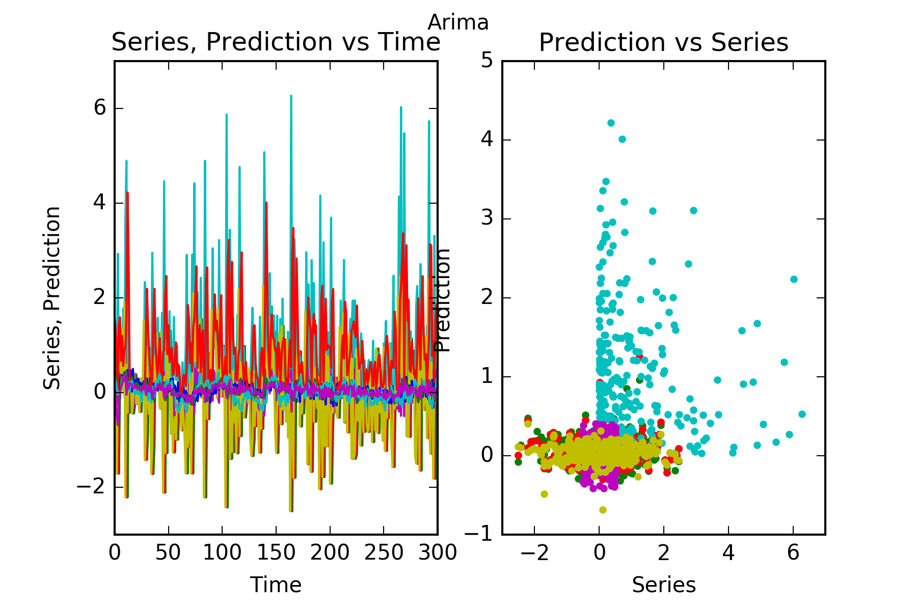
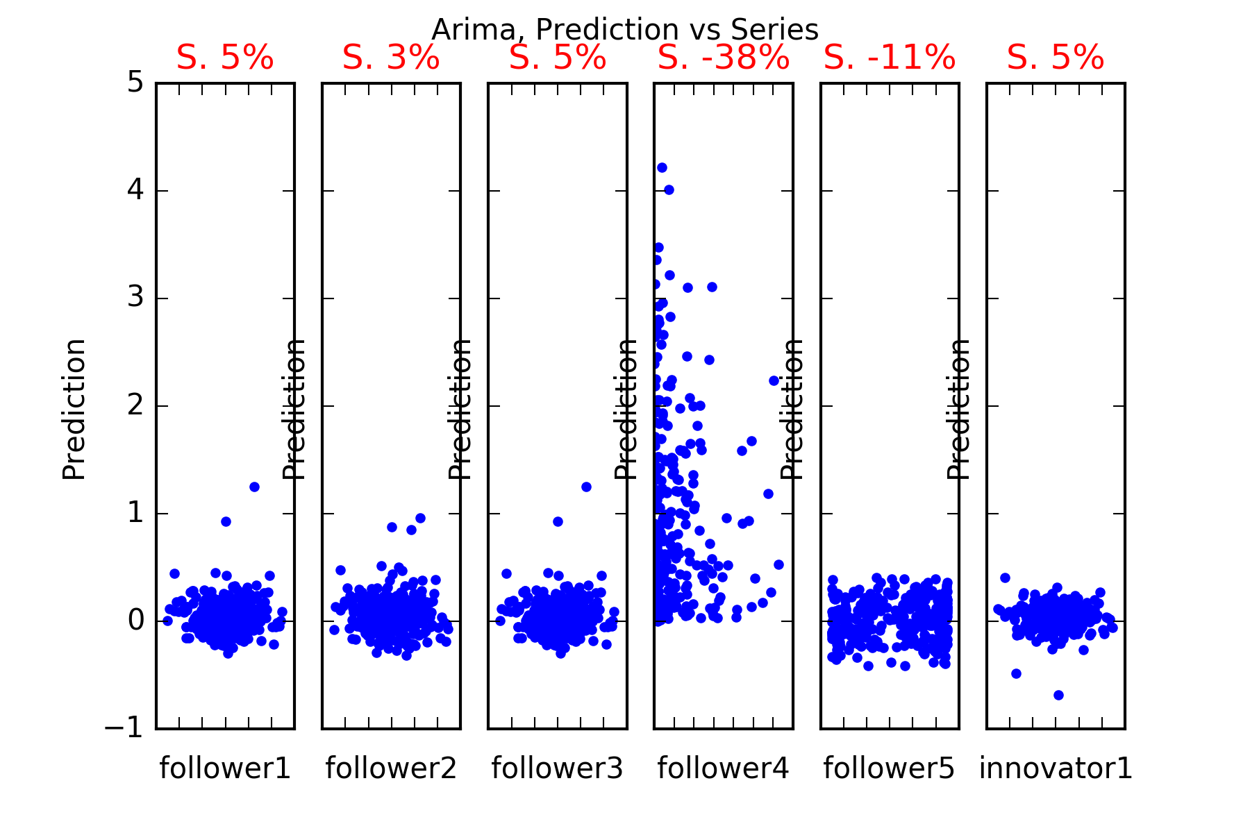
Interpretation : Arima does not beat our simple benchmark in any of the series, it can’t predict any of the other series follower1, follower2, follower3, follower4, follower5 or innovator1. This is evidenced in the figures, and also in the skill scores(Skill in the figures). A skill score of 100% implies perfect prediction, 0% skill score implies the prediction is as good as random chance.

Dense

As mentioned, the  defineFitPredict needs to be defined for each forecasting technique. In the case of our dense network we usedefineFitPredict_DENSE, which is also supplied by our package timeseries_utils.

Now we run the script shown above.

The model summary is this:

The result is:

 

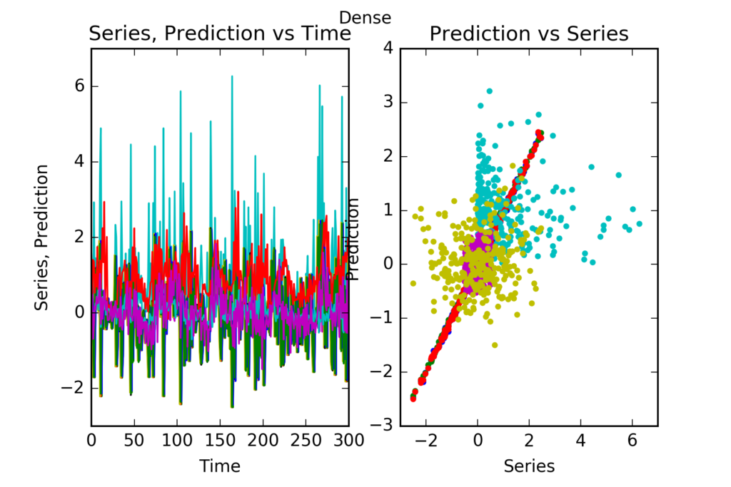
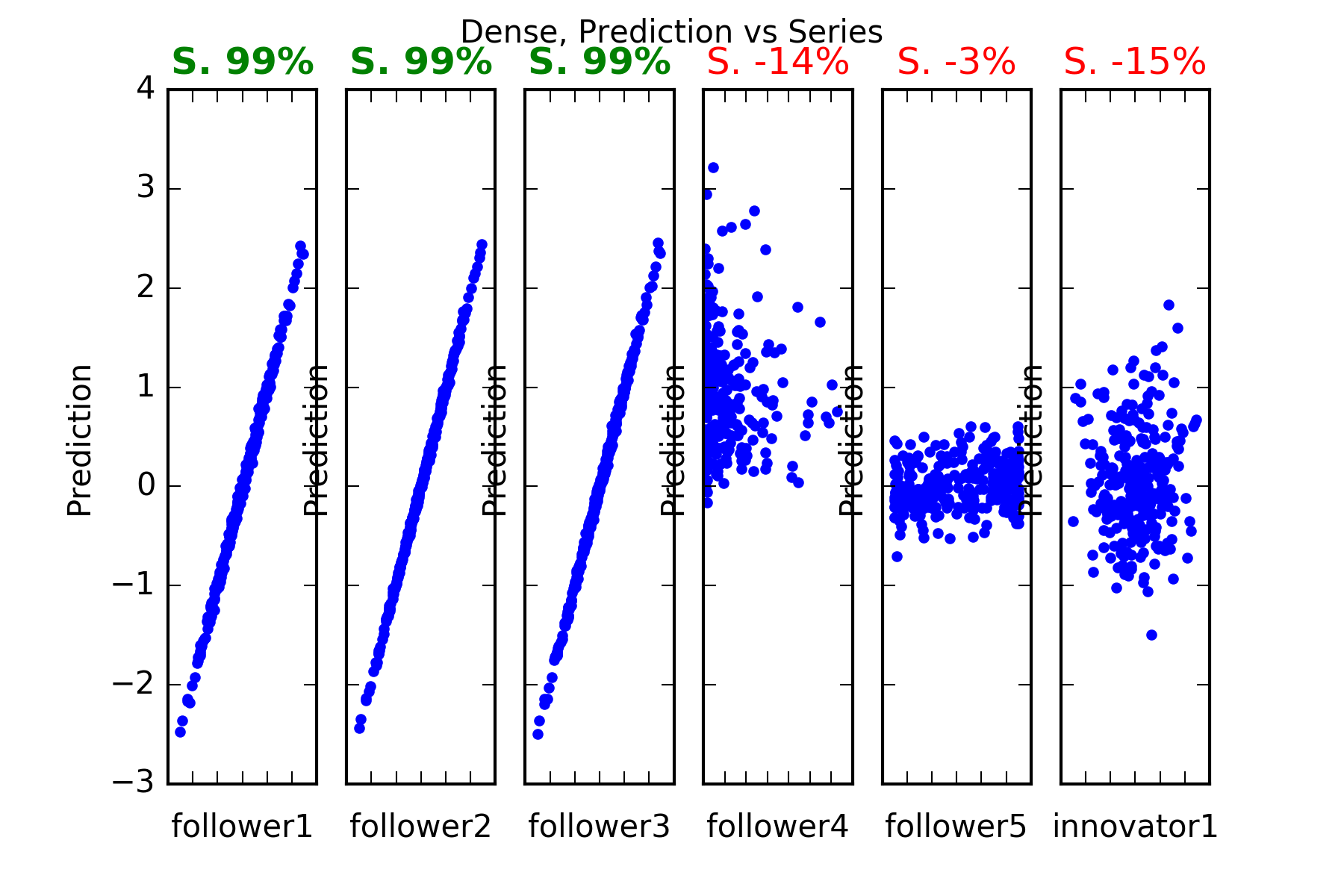
Interpretation : Dense  predicts perfectly follower1, follower2 and follower3. It can’t beat the reference becnhmark in the prediction of any of the other series follower4, follower5 or innovator1. This is evidenced in the figures, and also in the skill scores(called skill in the figures). A skill score of 100% means perfect prediction, 0% skill score means the prediction is as good as random chance. The series with significant skills are follower1, follower2 and follower3.

LSTM

As mentioned, the  defineFitPredict needs to be defined for each forecasting technique. In the case of our LSTM network we use defineFitPredict_LSTM, which is also supplied by our package timeseries_utils.

Now we run the script shown above.

The model summary is this:

The result is:

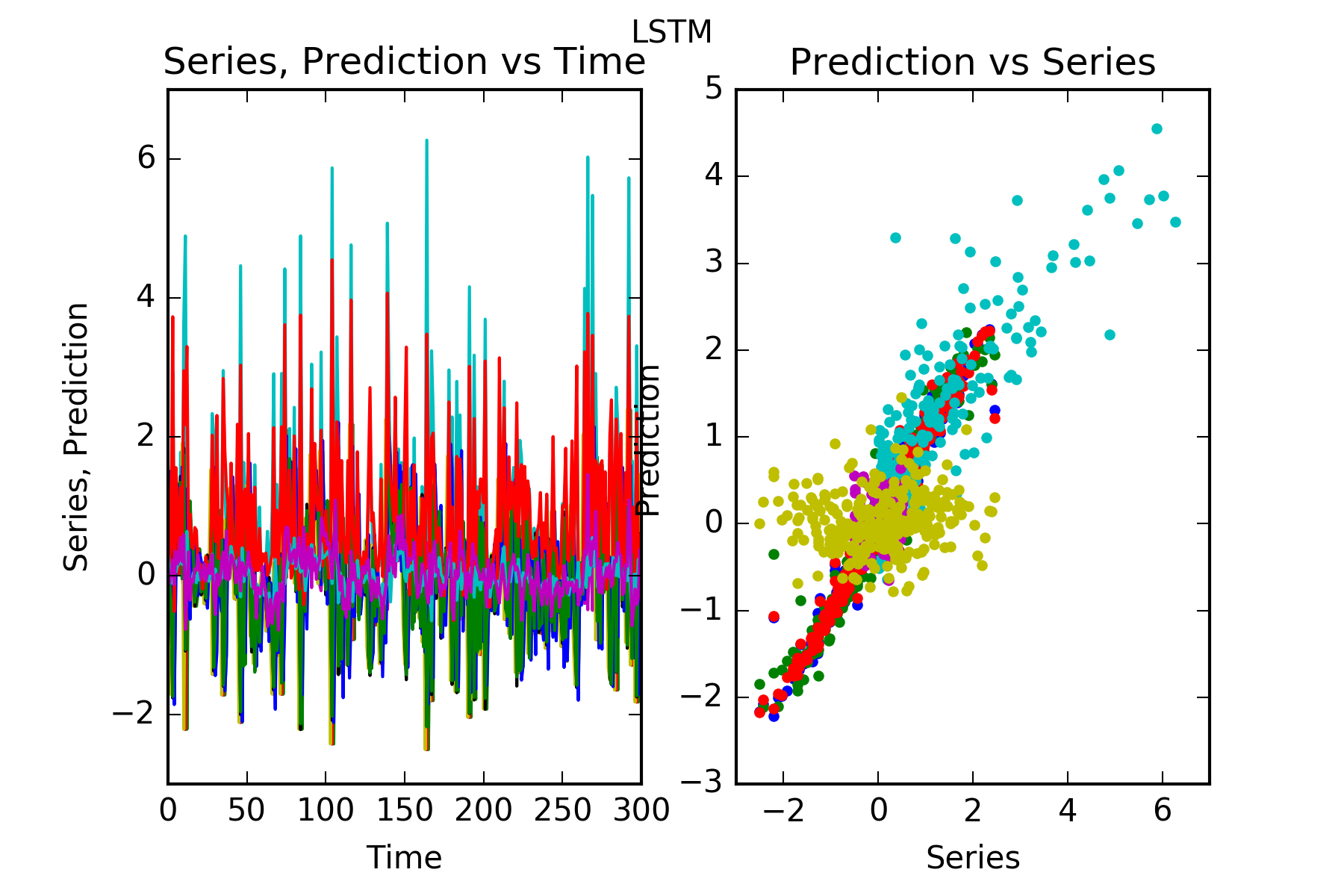
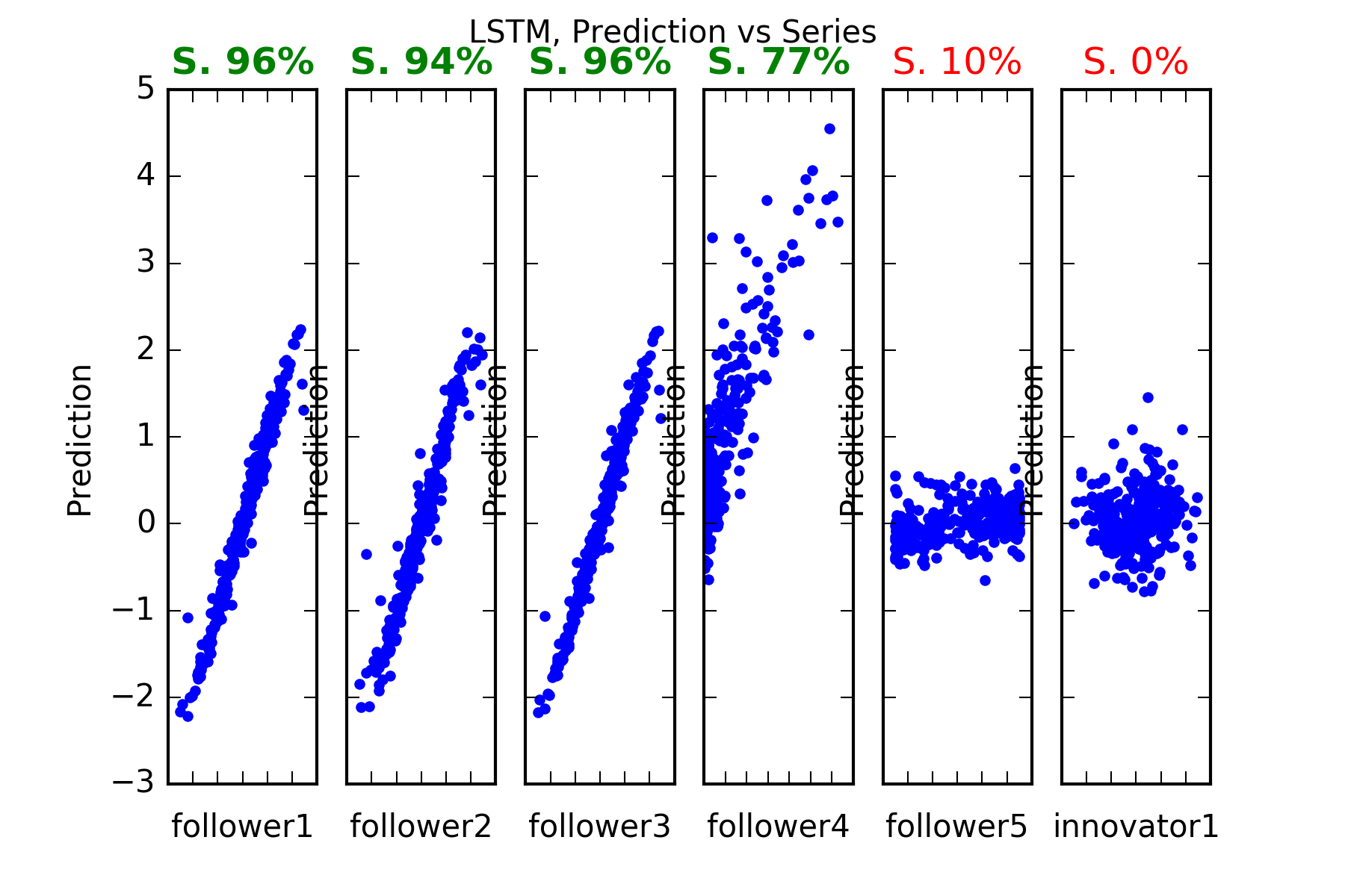
Interpretation : LSTM  predicts perfectly all the follower series that is follower1, follower2 and follower3, follower4. It can’t predict the unpredictable (if we believe our pseudo-random number generator is truly random) innovator1. This is evidenced in the figures, and also in the skill scores(called skill in the figures). A skill of 100% means perfect prediction, 0% skill score means the prediction is as good as random chance. The series with significant skills are follower1, follower2 and follower3, follower4.

Result summary:

Here’s the summary table:

Method/Timeseries	Arima	Dense	LSTM
follower1	✕	✔	✔
follower2	✕	✔	✔
follower3	✕	✔	✔
follower4	✕	✕	✔
follower5	✕	✕	✕
innovator1	✕	✕	✕

LSTM wins!