
In this follow up post we apply the same methods we developed previously to a different dataset.
Again, as previously, we make use of the out github hosted package timeseries_utils, and a script:
# load data
import os
os.chdir('** use your own dictionary, where you want to save your plots **')

# load packages and package-based-functions
import numpy as np
import matplotlib.pyplot as plt

from timeseries_utils import Configuration, Data
from timeseries_utils import calculateForecastSkillScore

# configuration
C = Configuration()

C.dictionary['nOfPoints'] = 600
# below 300 things dont work so nicely, so we use a value considerably above that
C.dictionary['inSampleRatio'] = 0.5

C.dictionary['differencingOrder'] = 1

C.dictionary['p_order'] = 7
C.dictionary['steps_prediction'] = 1

C.dictionary['epochs'] = 100
C.dictionary['verbose'] = 0

C.dictionary['modelname'] = modelname


# create data
# # set random seed for reproducibility
np.random.seed(178)
D = Data()
nOfSeries = 7

artificial_x, artificial_SERIES = artificial_data(nOfPoints = C.dictionary['nOfPoints'],
                                   nOfSeries = nOfSeries,
                                   f_rauschFactor = 0.5)


for S in range(nOfSeries):

    signal_S = 'signal' + str(S)
    D.setFollower(signal_S, otherSeries=artificial_SERIES[:,S], otherSeriesName='innovator plus' + signal_S)


SERIES_train = D.train(D.SERIES(), Configuration=C)
SERIES_test = D.test(D.SERIES(), Configuration=C)

VARIABLES_train = D.train(D.VARIABLES(), Configuration=C)
VARIABLES_test = D.test(D.VARIABLES(), Configuration=C)

#define, fit model; predict with with model
Prediction, Model = defineFitPredict(C=C,
                                     D=D,
                                     VARIABLES_train=VARIABLES_train,
                                     SERIES_train=SERIES_train,
                                     VARIABLES_test=VARIABLES_test,
                                     SERIES_test=SERIES_test)

# calculate Accuracy : 0% as good as NULL-Hypothesis, 100% is perfect prediction
Skill = calculateForecastSkillScore(actual=SERIES_test, predicted=Prediction, movingAverage=20)

# plot stuff
f, axarr = plt.subplots(1, 2, sharey=True)

f.suptitle(predictionModel)

axarr[0].plot(SERIES_test)
axarr[0].plot(Prediction)
axarr[0].set_title('Series, Prediction vs Time')
axarr[0].set_xlabel('Time')
axarr[0].set_ylabel('Series, Prediction')

axarr[1].plot(SERIES_test, Prediction, '.')
axarr[1].set_title('Prediction vs Series')
axarr[1].set_xlabel('Series')
axarr[1].set_ylabel('Prediction')

plt.savefig(plotname + '_1.png', dpi=300)
plt.show()
# end: # plot stuff


# second set of plots
f, axarr = plt.subplots(1, D.numberOfSeries(), sharey=True)

f.suptitle( predictionModel + ', Prediction vs Series')

seriesTitles = list(D.dictionaryTimeseries.keys())

x = 1


for plotNumber in range(D.numberOfSeries()):

    seriesNumber = plotNumber

    axarr[plotNumber].plot(SERIES_test[:,seriesNumber], Prediction[:,seriesNumber], '.')
#     axarr[plotNumber].plot(SERIES_test[:-x,seriesNumber], Prediction[x:,seriesNumber], '.')

    if Skill[seriesNumber] < 50:
        axarr[plotNumber].set_title('S. ' + str(Skill[seriesNumber]) + '%', color='red')

    if Skill[seriesNumber] > 50:
        axarr[plotNumber].set_title('S. ' + str(Skill[seriesNumber]) + '%', color='green', fontweight='bold')


    axarr[plotNumber].set_xlabel(seriesTitles[seriesNumber])
    axarr[plotNumber].set_ylabel('Prediction')
    axarr[plotNumber].set_xticklabels([])

plt.savefig(plotname + '_2.png', dpi=300)

plt.show()
# end: # second set of plots
Data
The main difference to the previous post is the data. In this post the data is again created artificially. However here, we use a collection of univariate series, which makes this setting particular suitable for arima. The univariate series are composed of composed of a random innovator part and a predictable part, with offsets.
In order for our skill score to be able to cope with the offsets, we need to use the a moving average model as the reference viz. null hypothesis. In this post we use a averaging window of one, as implied by movingAverage=1, which is just the actual series’ previous value.
Results
Arima
As mentioned, the defineFitPredict needs to be defined for each forecasting technique. In the case of arima we use defineFitPredict_ARIMA, which is supplied by our package timeseries_utils.
from timeseries_utils import artificial_data
from timeseries_utils import defineFitPredict_ARIMA, defineFitPredict_DENSE, defineFitPredict_LSTM

defineFitPredict = defineFitPredict_ARIMA
predictionModel = 'Arima'

modelname = predictionModel + '-Artificial'

plotname = 'forecasting_2_arima'
Now we run the script shown above.
The configuration is this:
The configuration is (in alphabetical order):

differencingOrder:1
epochs:100
inSampleRatio:0.5
...
nOfPoints:600
p_order:7
splitPoint:300
steps_prediction:1
verbose:0


The data summary is:

SERIES-shape:(600, 7)
signal0:{'follows': 'innovator plussignal0', 'shiftedBy': None}
signal1:{'follows': 'innovator plussignal1', 'shiftedBy': None}
signal2:{'follows': 'innovator plussignal2', 'shiftedBy': None}
signal3:{'follows': 'innovator plussignal3', 'shiftedBy': None}
signal4:{'follows': 'innovator plussignal4', 'shiftedBy': None}
signal5:{'follows': 'innovator plussignal5', 'shiftedBy': None}
signal6:{'follows': 'innovator plussignal6', 'shiftedBy': None}
The result is:
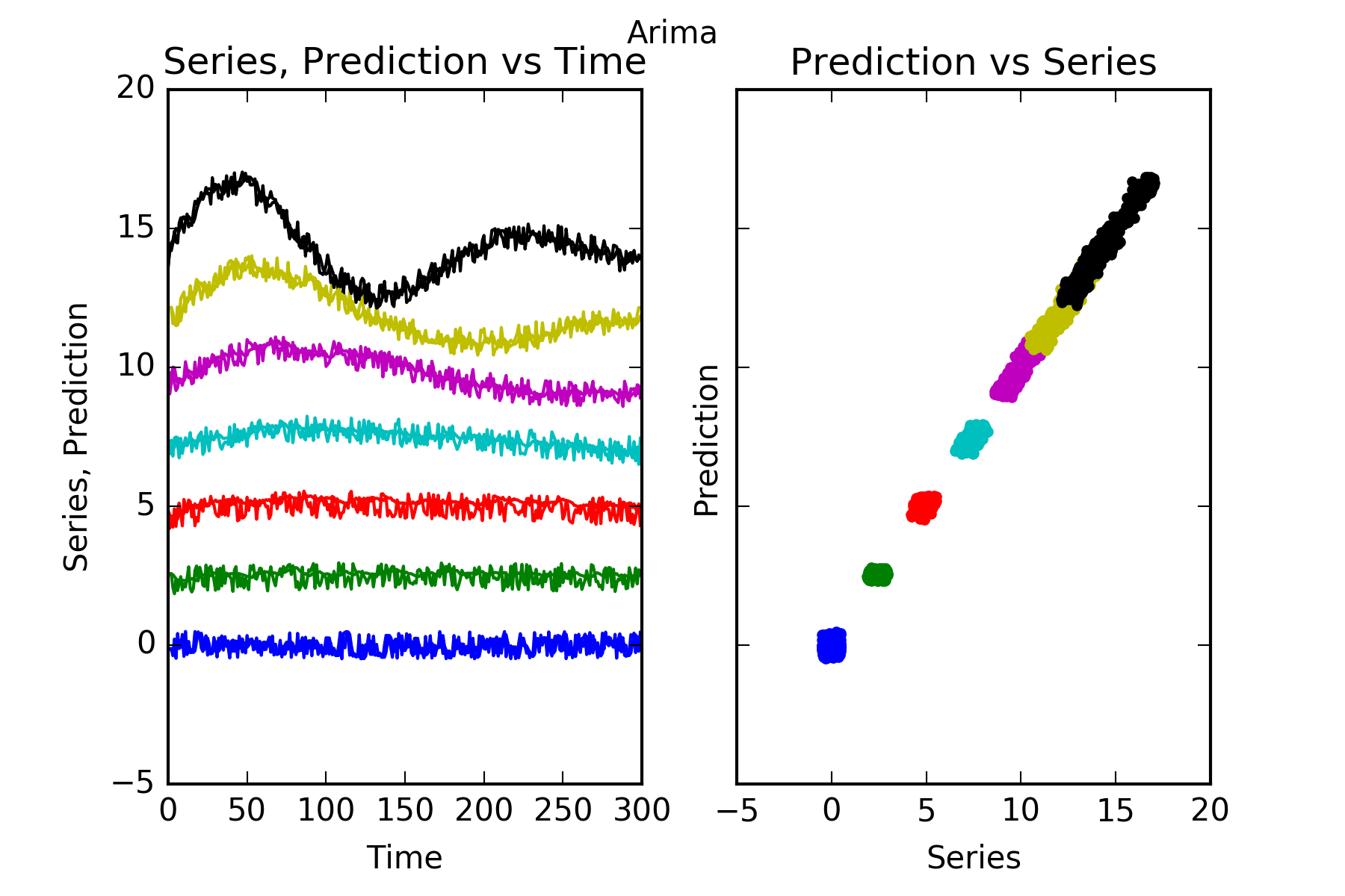
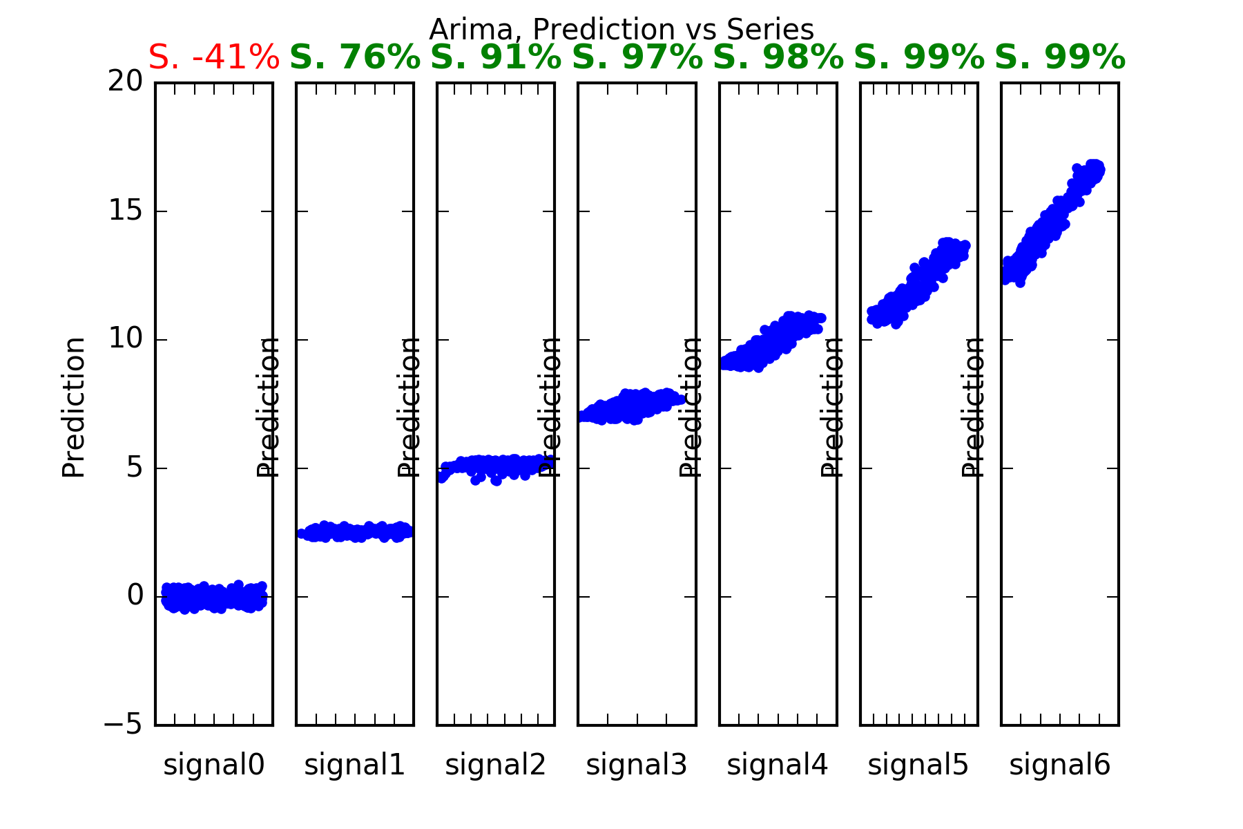
Interpretation : As noted above, Arima performs well in this setting, ie with data being a collection of univariate series. It predicts those series with predictable parts, ie series1 to series6. And it cannot predict signal0, which is a random noise innovator.
This is evidenced in the figures, and also in the skill scores(S. in the figures). An skill score of 100% means perfect prediction, 0% skill score means the prediction is as good the alternative reference hypothesis, for which here we have chosen the series’ lagged previous value.
Dense
As mentioned, the defineFitPredict needs to be defined for each forecasting technique. In the case of our dense network we usedefineFitPredict_DENSE, which is also supplied by our package timeseries_utils.
from timeseries_utils import artificial_data
from timeseries_utils import defineFitPredict_ARIMA, defineFitPredict_DENSE, defineFitPredict_LSTM

defineFitPredict = defineFitPredict_DENSE
predictionModel = 'Dense'

modelname = predictionModel + ' Artificial'

plotname = 'forecasting_2_dense'
Now we run the script shown above.
Note that we’ve turned on differencing, as is evident in the configuration with differencingOrder:1. This improves performance.
The model summary is this:
Layer (type)                 Output Shape              Param #
=================================================================
dense_1 (Dense)              (None, 7, 64)             512
_________________________________________________________________
flatten_1 (Flatten)          (None, 448)               0
_________________________________________________________________
dropout_1 (Dropout)          (None, 448)               0
_________________________________________________________________
dense_2 (Dense)              (None, 7)                 3143
=================================================================
Total params: 3,655
Trainable params: 3,655
Non-trainable params: 0
_________________________________________________________________
The result is:
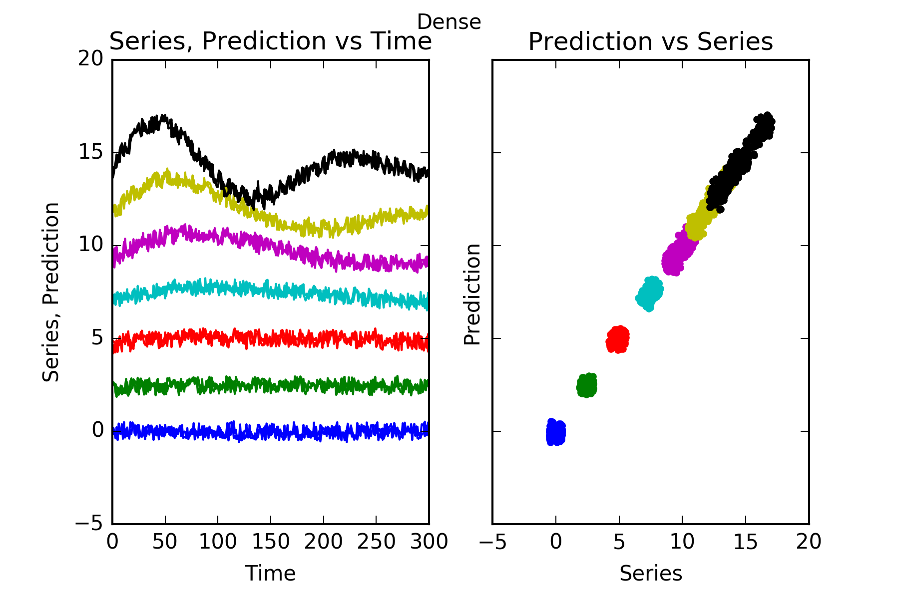

Interpretation : The performance of the Dense prediction is on par with Arima’s.
Its prediction beats the benchmark for those series with predictable parts, ie series1 to series6. And it certainly cannot predict signal0, which is a random noise innovator.
This is evidenced in the figures, and also in the skill scores(Acc. in the figures). An skill score of 100% means perfect prediction, 0% skill score means the prediction is as good as random chance. As stated the only series where the skill is close to 0, is series signal0.
LSTM
The model summary is this:
_________________________________________________________________
Layer (type)                 Output Shape              Param #
=================================================================
lstm_1 (LSTM)                (None, 16)                1536
_________________________________________________________________
dense_1 (Dense)              (None, 7)                 119
=================================================================
Total params: 1,655
Trainable params: 1,655
Non-trainable params: 0
_________________________________________________________________
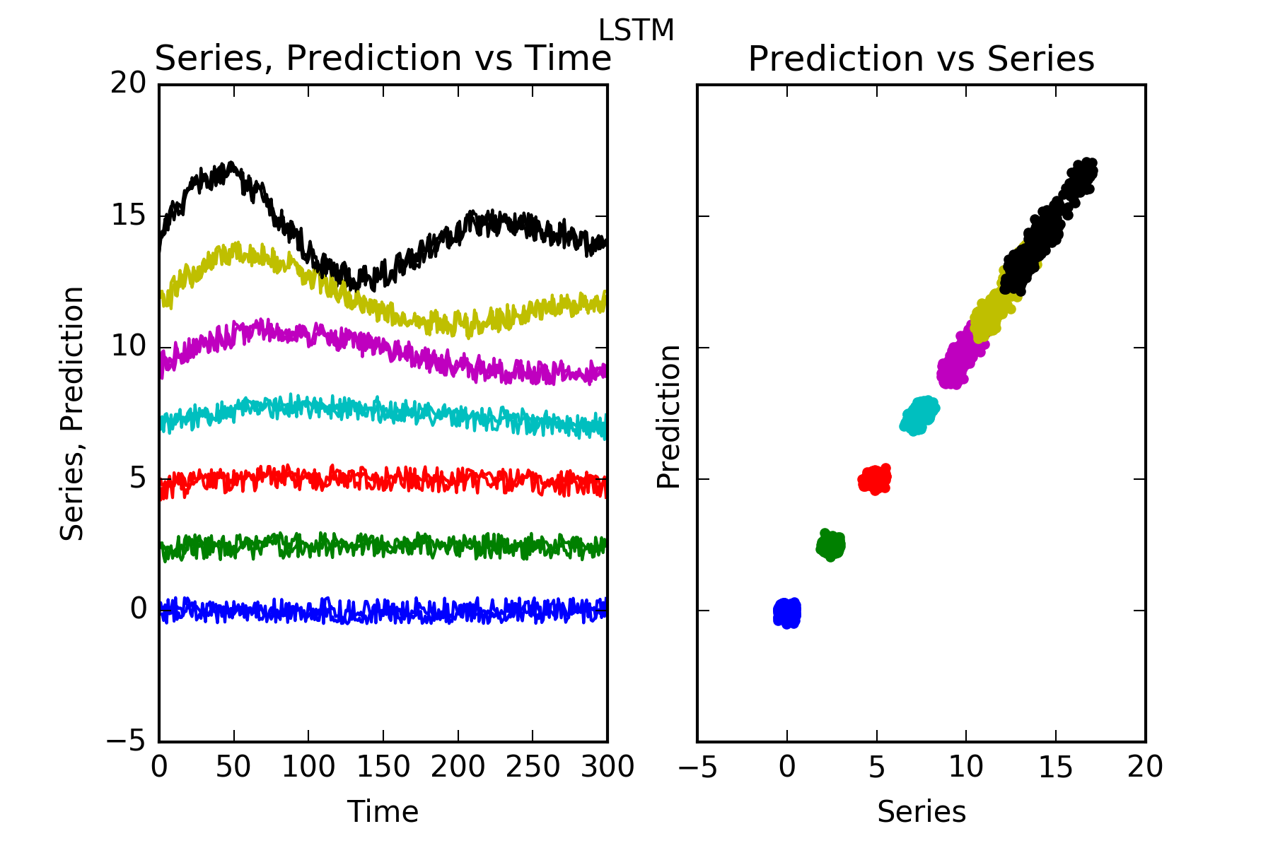
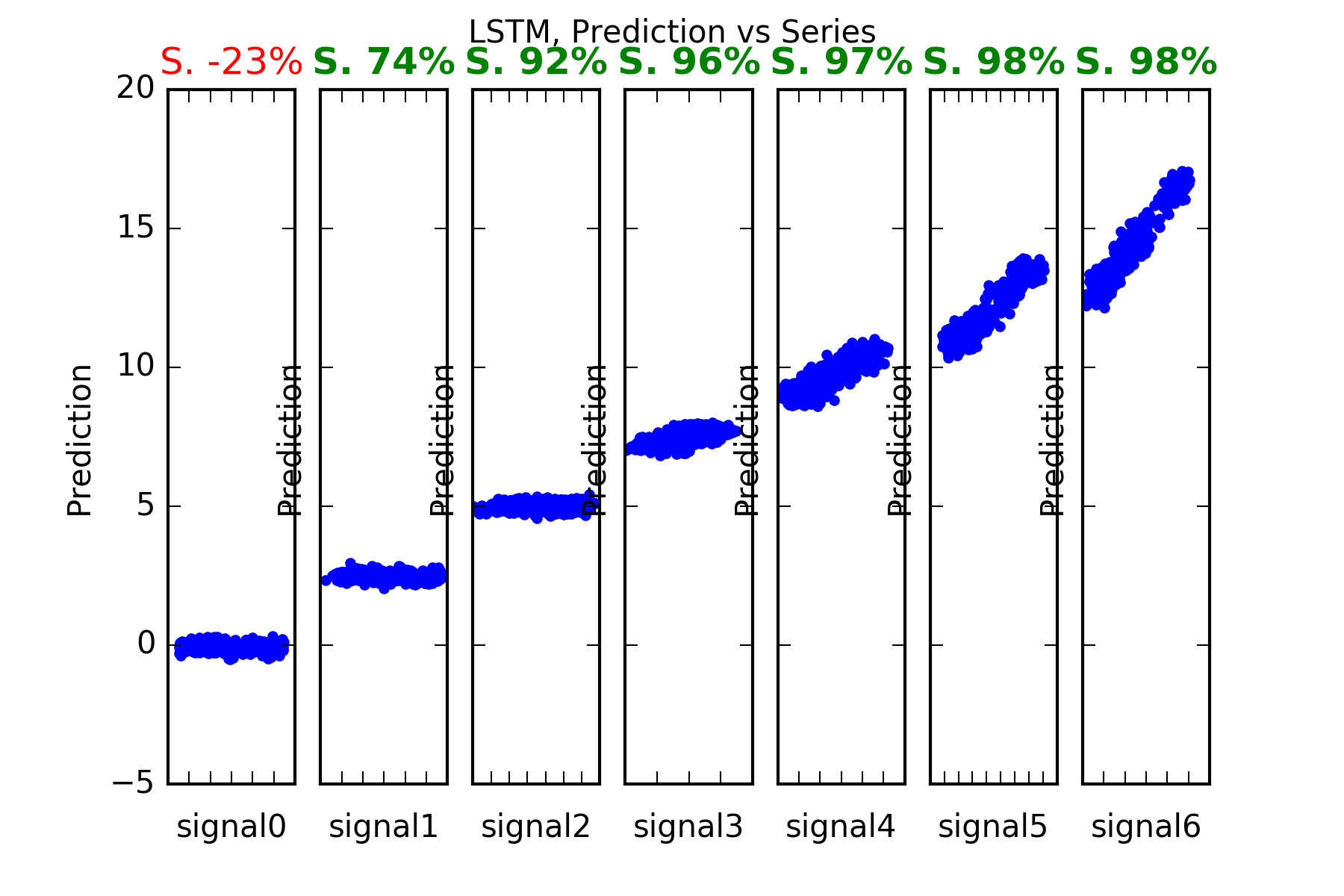
Interpretation : Except for the nearly unpredictable signal0, the performance of the Dense prediction is on par with Arima’s and Dense’s.
Its prediction beats the benchmark for those series with predictable parts, ie series1 to series6. And it certainly cannot predict signal0, which is a random noise innovator.
This is evidenced in the figures, and also in the skill scores(S. in the figures). A skill score of 100% means perfect prediction, 0% skill score means the prediction is as good as random chance. As stated the only series where the sklill is close to 0, is series signal0.
Result summary:
Here’s the summary table:
| Method/Timeseries | Arima | Dense | LSTM |
|---|---|---|---|
| signal0 | ✕ | ✕ | ✕ |
| signal1 | ✔ | ✔ | ✔ |
| signal2 | ✔ | ✔ | ✔ |
| signal3 | ✔ | ✔ | ✔ |
| signal4 | ✔ | ✔ | ✔ |
| signal5 | ✔ | ✔ | ✔ |
| signal6 | ✔ | ✔ | ✔ |
There is no clear winner with this data, which is composed of a collection of univariate series. We have three joint winners: Arima, Dense and LSTM.