
This post is a follow-up of 1.
We start off with an eye-catching plot, representing the functioning of an optimiser using the stochastic gradient method. The plot is explained in more detail further below.
Visualisation of a loss surface with multiple minima. The surface is in gray, the exemplary path taken by the optimiser is in colors.
We had previously explored a visualisation of gradient-based optimisation. To this end we plotted an optimisation path against the background of its corresponding loss surface.
Remark: the loss surface is a function that is typically used to describe the badness of fit of an optimisation.
Following the logic of a tutorial from tensorflow2 , in the previous case we looked at a very simple optimisation, maybe one of the simplest of all : we used linear regression. As data points we used a straight line with mild noise (= a little bit of noise, but not too much). Further, we used the offset and the inclination as fitting parameters. As a loss function we used a quadratic function, which is very typical. It turns out that this produces a very well behaved loss surface, with a simple valley, which the optimiser has no problem of finding.
As a special case, the surface can be one-dimensional. In this current post, for simplicity, we use only one optimisation parameter, therefore the surface is one-dimensional. The fitting parameter we use here is the straight line’s angle. Despite this one-dimensional simplicity, we construct a surface which is reasonably hard for the gradient-based optimiser, and in fact can derail it.
The primary purpose of this post is to construct from artificial data and visualise a loss surface that is not well behaved, and which in particular has many minima.
As usual, the code can be found on github (in a jupyter notebook):
Remark : The static plots can be viewed by opening the jupyter file from github, even without executing it.
Requirements
Hardware
- A computer with at least 4 GB Ram
Software
- The computer can run on Linux, MacOS or Windows
- Familiarity with Python
Let’s get started
We provide a notebook which is is a derived from one the previous post’s notebooks 01 – Custom_training_basics_standard_optimizer_multiple_valleys.ipynb.
The name-part “multiple_valleys” is an indication of the primary purpose of this post: to construct from artificial data and visualise a loss surface that is not well behaved, and which in particular has many minima.
There are more details in the notebook, so here I will keep things short and just provide additional comments.
Data
The data are several intersecting straight lines:
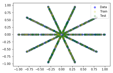
The data set has obvious rotational symmetry, so this should already produce a loss surface with several minima. True?
This is true if there is a minimum associated with any of the straight lines of the rosette/bundle/bushel. However this is not the case for the quadratic loss function. For the quadratic loss function things are still well behaved.
Why is this so? (You can try to think about this for a minute, it’s a little brain teaser).
Answer: Because the larger errors dominate. So we have to tweak the loss function to make the smaller errors count.
For the tweaked loss function we use:
loss_function_tweak = 4

def loss(predicted_y, desired_y):
  return tf.reduce_mean(((predicted_y - desired_y)**2)**(1/loss_function_tweak))
There are other possibilities to do this, in fact infinitely many. The main point is to make the function sublinear. This purpose is served by the use of the 4-th root.
Data fit

For the optimisation, the data is split into train and test data.
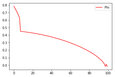
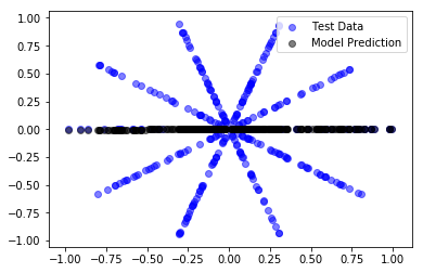
To keep things as simple as possible we only look at straight lines going through the origin, and only search for the best solution by varying the angle (phi).
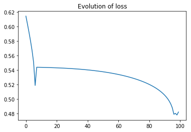
We stopped the optimisation after 100 steps. Because the surface is “difficult”, the simple gradient scheme, has difficulties dealing with it, which means, that it does not always go from good to better. Instead, occasionally when it has come quite close, it is derailed and gets worse. In between the optimisation algorithm focuses on one of the straight lines. This is in fact the behaviour we expect, because we use a sublinear loss-function, which sub-proportionally weights errors. It tries to avoid the smaller errors as much as it can, against a background of larger errors that only count relatively little.
Conclusion
We have successfully constructed and visualised a loss surface with multiple minima, arising from a combination of
- simple artificial data set example, consisting of a dataset of a rosette/bundle/bushel of intersecting lines,
- which we try to fit with a straight line,
- the avoidance of noise in the data-set helps to show more pronounced features.
- Further the loss function needs to be selected carefully, especially good for the current purpose are sub-linear loss functions.