
There are entire theses devoted to reinforcement learning of the game of nim, in particular those of ERIK JÄRLEBERG (2011) and PAUL GRAHAM & WILLIAM LORD (2015).
Those two were successful in training a reinforcement-based agent to play the game of nim with a high percentage of accurate moves. However, they used lookup tables as their evaluation functions, which leads to scalability problems. Further, there is no particular advantage in using Q-learning as opposed to a Value-based approach. This is due to the fact that the “environment’s response” to a particular action (“take b beans from heap h”) is entirely known, and particularly simple. This is different, e.g. from games where the rules are unclear and not stated explicitly and must be learned by the agent, as is the case in the video. In the game of nim the rules are stated explicitly. Indeed, if the action “take b beans from heap h” is possible, i.e. there are at least b beans on heap h, then the update rule is:
heapSize(h) -> heapSize(h) – b
In other the size of heap h is reduced by he beans taken away from it. Therefore, as stated, there is no advantage in using Q-learning over a Value-based approach. The curse of dimensionality, however, is worse for the Q-learning setup as for a heap vector of (h0, h1, …, hn-1) there is one Value but, without paying special attention to duplicates,
~ h0* h1 * … * hn-1 actions, and therefore ~ h0* h1 * … * hn-1 Q-values. There will use a Value based approach.
In other words, we want to use a neural network approximation for the evaluation function. A priori, it is, however, by no means clear that this type of function approximation will work. Yet, the game of Nim is in a sense easy, as there is a complete solution of the game. We can use this solution to our advantage by using it to estimate whether it is likely that the mentioned network approximation will work.
A simple way is to use supervised learning as a test.
The simplest case is to test a classification of a position as winning or losing.
Can a simple neural network be trained to learn whether a nim position is winning or losing?
The out-of-sample probability of correct classification is an estimate of the upper bound of the same learning task being achieved by reinforcement.
To specify the network we use keras with tensorflow as the backend. Keras is a high-level specification, which is very convenient.
An example of a network specification may look like this:
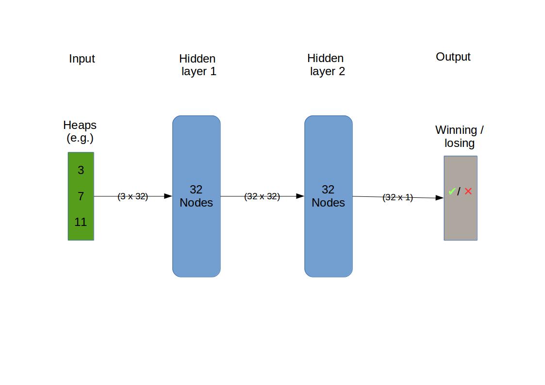
model = Sequential(    )

model.add(Dense(units = 32, input_shape = (3,), activation='sigmoid'))
model.add(Dense(units = 32, activation='sigmoid'))
model.add(Dense(units = 1, activation='sigmoid'))

model.compile(optimizer='adam', loss='binary_crossentropy', metrics=['binary_accuracy'])
So the expected input is a 3-vector specifying the heap sizes. The output is binary i.e. True if winning, False if losing. There are three hidden layers with 32 nodes. Nodes are also called connected units or artificial neurons. The optimizer is adam (“adaptive moment estimation”), which is a sophisticated version of stochastic gradient descent (“SGD”), which itself is the standard method of optimising the fit a neural network delivers.
To find a a network that performs reasonably well, we must look at various alternatives for the choice of network, a process also known as hyperparameter optimisation. This involves looking at how well and after how much training a given network performs for values it has not been trained with, this is called “out of sample”.
To track this, we need to look at the history of training. Keras provides a function for that purpose. However, the history is lost between sessions and also when the optimisation is restarted. Therefore we use a wrapper class for the model to provide this functionality, namely to persistently save and merge model histories. The wrapper class is based on this.
#!/usr/bin/env python3
# -*- coding: utf-8 -*-
"""
Created on Wed Jan  3 11:21:22 2018

@author: hfwittmann
"""

# https://github.com/keras-team/keras/issues/103

from keras.models import Sequential
from keras.models import load_model

from collections import defaultdict

import pickle
from pathlib import Path

from IPython.core.debugger import set_trace


def _merge_dict(dict_list):
    dd = defaultdict(list)
    for d in dict_list:
        for key, value in d.items():
            if not hasattr(value, '__iter__'):
                value = (value,)
            [dd[key].append(v) for v in value]
    return dict(dd)

def save(obj, name):
    try:
        filename = open(name + ".pickle","wb")
        pickle.dump(obj, filename)
        filename.close()
        return(True)
    except:
        return(False)

def load(name):
    filename = open(name + ".pickle","rb")
    obj = pickle.load(filename)
    filename.close()
    return(obj)

def load_model_w(name):
    # load if exists
    my_file = Path(name)

    # set_trace()

    if my_file.is_file():
        # file exists
        model_k = load_model(name)
        model = Sequential_wrapper(model_k)

        history = load(name)
        model.history = history

        return(model)


class Sequential_wrapper():
    """
    %s
    """%Sequential.__doc__

    def __init__(self, model=Sequential()):
        self.history = {}
        self.model = model

        # method shortcuts
        methods = dir(self.model)
        for method in methods:
            if method.startswith('_'): continue
            if method in ['model','fit','save']: continue
            try:
                exec('self.%s = self.model.%s' % (method,method))
            except:
                pass

    def _update_history(self,history):
        if len(self.history)==0:
            self.history = history
        else:
            self.history = _merge_dict([self.history,history])

    def fit(self, x, y, batch_size=32, epochs=10, verbose=1, callbacks=None,
            validation_split=0.0, validation_data=None, shuffle=True,
            class_weight=None, sample_weight=None,
            initial_epoch=0, **kwargs):
        """
        %s
        """%self.model.fit.__doc__
        h = self.model.fit(x, y, batch_size, epochs, verbose, callbacks,
                     validation_split, validation_data, shuffle,
                     class_weight, sample_weight,
                     initial_epoch, **kwargs)
        self._update_history(h.history)
        return h

    def save(self, filepath, overwrite=True):
        """
        %s
        """%self.model.save.__doc__
        save(self.history,filepath)
        self.model.save(filepath, overwrite)
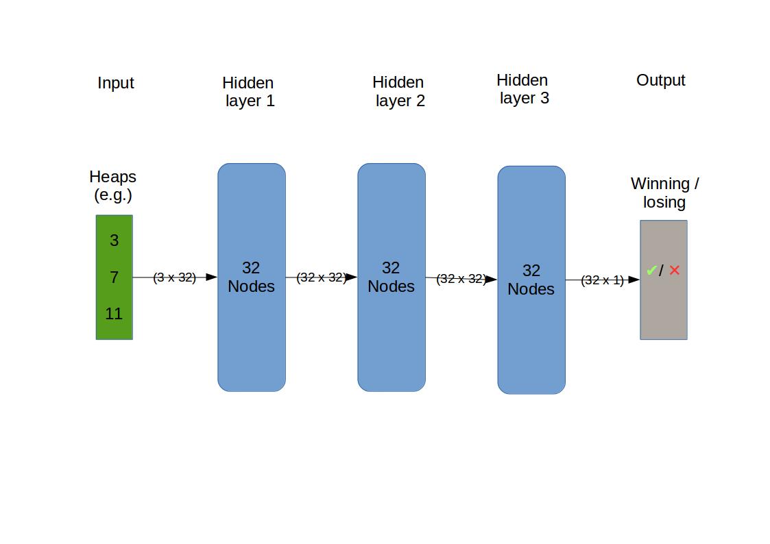
We focus our attention on a family of networks that are distinguished solely by the number of intermediate layers that are inserted between the input and output layers. For the intermediate layers we specify the same form, namely 32 nodes with sigmoid activation.
#!/usr/bin/env python3
# -*- coding: utf-8 -*-
"""
Created on Sun Dec 31 17:57:17 2017

@author: hfwittmann

Supervised learning of winning / losing positions
"""

import numpy as np
from nim_perfect_play.nim_perfect_play import findWinningMove

import matplotlib.pyplot as plt

from keras.models import Sequential
from keras.layers import Dense
from keras.optimizers import *

from track_model_history import Sequential_wrapper, load_model_w


# config
maxHeapSize = 7 # 20
shape = [10000, 3]

np.random.seed(167)
# positions
random_positions = np.random.random_integers(1,maxHeapSize, size = shape)

# intialize
next_positions = np.zeros(shape = shape)
winning_from_random = np.zeros(shape[0], dtype = bool )
winning_from_next = np.zeros(shape[0], dtype = bool )
move_from_random = np.zeros([shape[0], 2])

# https://stackoverflow.com/questions/5347065/interweaving-two-numpy-arrays

for heapIndex in np.arange(len(random_positions)):

    #  to debug
    #    heapIndex = 0

    heap = random_positions[heapIndex]

    fWM = findWinningMove(heap)

    next_positions[heapIndex] = fWM['next_position']
    winning_from_random[heapIndex] = fWM['winning']
    winning_from_next[heapIndex] = not fWM['winning']
    move_from_random[heapIndex] = fWM['move']


positions = np.empty(shape = [ shape[0] * 2, shape[1] ])
positions[0::2,:] = random_positions
positions[1::2,:] = next_positions

winning = np.empty(shape = shape[0] * 2)
winning[0::2] = winning_from_random
winning[1::2] = winning_from_next


def buildNetwork(numberOfLayers):


    model = Sequential(    )
    model.add(Dense(units = 32, input_shape = (shape[1],), activation='sigmoid'))

    for n in range(numberOfLayers):
        model.add(Dense(units = 32, activation='sigmoid'))

    model.add(Dense(units = 1, activation='sigmoid'))

    model.compile(optimizer='adam', loss='binary_crossentropy', metrics=['binary_accuracy'])

    return model


for numberOfLayers in range(3):

    filenName = "cache/nim-supervised" + "-32" * numberOfLayers +".h5"

    previousModel = load_model_w(filenName)

    if previousModel:
        model = previousModel
    else:
        model = buildNetwork(numberOfLayers)

    ModelWrapper = Sequential_wrapper(model)


    #combine random_positions and next_positions

    ModelWrapper.fit(x = positions, y = winning, shuffle= 'batch', epochs = 1000, validation_split=0.1 )


    ModelWrapper.save(filenName)


    plt.plot(ModelWrapper.history['binary_accuracy'], label = 'In-Sample' + '_32' * numberOfLayers )
    plt.plot(ModelWrapper.history['val_binary_accuracy'], label = 'Validation_' + '_32' * numberOfLayers )


plt.legend(loc='best')
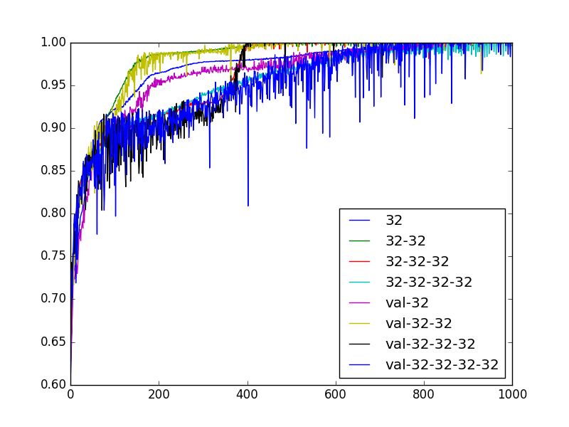
After a little experimentation, as detailed further below, we find a network that performs very well, if we limit the maximum heap size. A maximum heap size of 7 is good for us as a simple enough network leads to a nearly perfect performance.
After running for a while we have the an in and out-of-sample prediction accuracy of >99% (in fact 100%)
Next we try the same approach with a maximum heap size of 20, we call this setup 3 x max 20, to test the scalability of this family of networks.
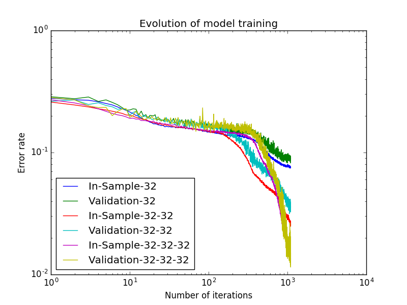
The results for 3 x max 7 and 3 x max 20 conform to some natural expectations we may have:
- The advantages of a deeper network become apparent for the larger heap sizes of up to twenty. This seems natural as here things are more complicated, which calls for a higher degree of abstraction, which in turn might be expected to be delivered by a deeper network.
- This abstraction by the deeper network comes at a price. As is apparent the training of the deeper network needs more iterations, each iteration is also slightly slower.
Conclusion
The initial question was : “Can a simple neural network be trained to learn whether a nim position is winning or losing?” The answer is yes. Both 32-32 and 32-32-32 seem good candidates for the function approximation part in reinforcement learning.
Important points:
- The majority of randomly chosen positions in the game of nim are won. To train the network effectively it is important to have a balanced mix of winning and losing positions.
- Playing an optimal move from a winning position leads next (by definition) to a lost position for the opponent.
- We use both the random positions and the (optimally chosen) next positions to achieve the desired balanced mix.
- We interweave the random positions and their next positions to make optimal use of the keras shuffling strategy that is batch-based.
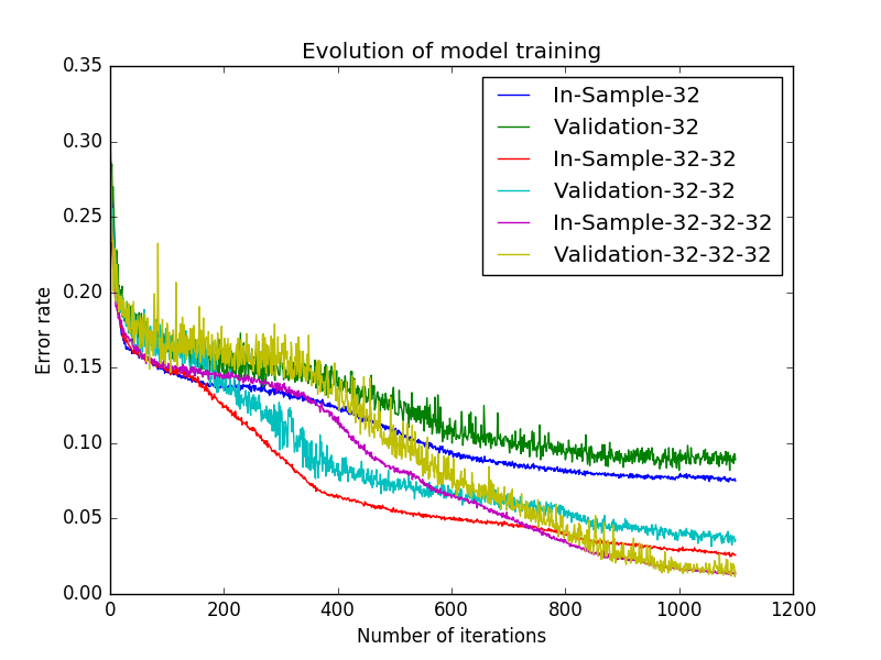
- In the training process we observe that the prediction accuracy of in-sample and out-of-sample mount in sync during the model-fitting process. This is important as it shows that the network generalises sufficiently well. This means that it is able to predict whether a position is winning or not, and this for positions that it has not seen before almost equally well as for those that it explicitly used in the fitting.
- The supervised method is available because the game of nim is solved (and has been for a long time). This is a luxury which permits a short cut to selecting a neural-network-based function approximation that works in the supervised case and therefore is likely to work in the reinforcement case, too. In games and other settings where the solution is not known, there is much more overhead in choosing the model, which means longer running times etc.