This is a follow up to https://arthought.com/comparison-of-a-very-simple-regression-in-tensorflow-and-keras/
It covers the same topic but in pytorch.
Remarks
This notebook is a pytorch-implementation based on a Tutorial notebook on the tensorflow web site.
- Custom training: basics | TensorFlow. TensorFlow. https://www.tensorflow.org/tutorials/eager/custom_training. Published December 17, 2018. Accessed December 29, 2018.
You can find some more insformation on eager execution, also on Tensorflow’s website: 2. Eager Execution | TensorFlow. TensorFlow. https://www.tensorflow.org/guide/eager. Published December 12, 2018. Accessed December 29, 2018.
We have marked sections that have differences with the original workbook in yellow.
Author: H. Felix Wittmann
There is no association between the author and Tensorflow.
#@title Licensed under the Apache License, Version 2.0 (the "License");
# you may not use this file except in compliance with the License.
# You may obtain a copy of the License at
#
# https://www.apache.org/licenses/LICENSE-2.0
#
# Unless required by applicable law or agreed to in writing, software
# distributed under the License is distributed on an "AS IS" BASIS,
# WITHOUT WARRANTIES OR CONDITIONS OF ANY KIND, either express or implied.
# See the License for the specific language governing permissions and
# limitations under the License.
Custom training: basics
import torch
assert torch.tensor(1.0) == 1.0, "Converting 1.0 to torch tensor, should match"
assert torch.tensor(1.0).numpy() == 1.0, "Converting 1.0 to torch tensor, then back to numpy, should match"
Define torch model
class Net(torch.nn.Module):
    def __init__(self: torch.nn):
        super(Net, self).__init__()


        mylayer = torch.nn.Linear(1,1)
        # initialise values .. to make results deterministic
        mylayer.bias = torch.nn.Parameter(torch.tensor([0.0]))
        mylayer.weight = torch.nn.Parameter(torch.tensor([[5.0]]))

        self.net = torch.nn.Sequential(
            mylayer
        )

    def forward(self: torch.nn, x):
        return self.net(x)
Check initialisation
myNet = Net()
# https://discuss.pytorch.org/t/how-to-print-models-parameters-with-its-name-and-requires-grad-value/10778
for name, param in myNet.named_parameters():
    if param.requires_grad:
        print (name, param.data)
net.0.weight tensor([[5.]])
net.0.bias tensor([0.])Obtain training data
Let’s synthesize the training data with some noise.
import numpy as np
nOfDatapoints = 1000
W_TRUE, b_TRUE = 3.0, 2.0
np.random.seed(314)
inputs = np.random.normal(size=nOfDatapoints)
noise = np.random.normal(size=nOfDatapoints)
outputs = W_TRUE * inputs + b_TRUE + noise
Split into train/test
from sklearn.model_selection import train_test_split
inputs_train, inputs_test, outputs_train, outputs_test = \
    train_test_split(inputs, outputs, test_size=0.33, random_state=42)
# outputs = outputs.reshape(-1,1)  # reshape to match keras output
import matplotlib.pyplot as plt
from jupyterthemes import jtplot
jtplot.style()
plt.scatter(inputs,outputs,c='b', alpha=0.5, label='Data')
plt.scatter(inputs_train, outputs_train, c='y', alpha=0.2, label='Train')
plt.scatter(inputs_test, outputs_test, c='g', alpha=0.2, label='Test')
plt.legend()## Explore data und Model<matplotlib.legend.Legend at 0x11c109f28>Explore data und Model before training
Before we train the model let’s visualize where the model stands right now. We’ll plot the model’s predictions in black and the testting data in blue.
mynet = Net()

prediction_test = mynet(torch.Tensor([inputs_test]).transpose_(0, 1)).detach().numpy()
plt.scatter(inputs_test, outputs_test, c = 'b', alpha=0.5, label = 'Test Data')
plt.scatter(inputs_test, prediction_test, c = 'k', alpha=0.5, label = 'Initial Model Guess')
plt.legend()
plt.show()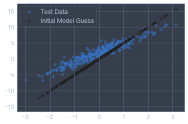
Set up loss function
from tensorboardX import SummaryWriter

objective = torch.nn.MSELoss(reduce=True)
optimizer = torch.optim.SGD(params=mynet.parameters(), lr=0.1)
writer = SummaryWriter(comment='-regression-tutorial')
Check
prediction_v = mynet( torch.Tensor([inputs_test]).transpose_(0,1))
outputs_v = torch.Tensor([outputs_test]).transpose_(0,1)
objective(prediction_v, outputs_v), ((outputs_v- prediction_v)**2).mean(), ((outputs_test.reshape(-1,1)- prediction_test)**2).mean()
(tensor(9.3949, grad_fn=<MseLossBackward>),
tensor(9.3949, grad_fn=<MeanBackward1>),
9.394942704256383)Do optimisation
batchsize = len(inputs_train)
epochs = 10
for ix in range(epochs):
    optimizer.zero_grad()
    prediction_v = mynet( torch.Tensor([inputs_train]).transpose_(0,1))
    outputs_v = torch.Tensor([outputs_train]).transpose_(0,1)

    loss_v = objective(prediction_v, outputs_v)
    loss_v.backward()
    optimizer.step()

    print("%d: loss=%.3f" % (ix, loss_v.item()))
    writer.add_scalar('loss', loss_v.item(), ix)
0: loss=9.306
1: loss=6.285
2: loss=4.368
3: loss=3.151
4: loss=2.379
5: loss=1.889
6: loss=1.578
7: loss=1.380
8: loss=1.255
9: loss=1.175
Explore data und Model after training
Before we train the model let’s visualize where the model stands right now. We’ll plot the model’s predictions in black and the testting data in blue.
prediction_test = mynet(torch.Tensor([inputs_test]).transpose_(0, 1)).detach().numpy()
plt.scatter(inputs_test, outputs_test, c = 'b', alpha=0.5, label = 'Test Data')
plt.scatter(inputs_test, prediction_test, c = 'k', alpha=0.5, label = 'Initial Model Guess')
plt.legend()
plt.show()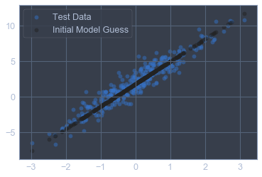
The notebook on GitHub: https://github.com/hfwittmann/comparison-tensorflow-keras/blob/master/04%20-%20Custom_training_basics_standard_optimizer_pytorch.ipynb